
CYCLISTIC BIKE-SHARE CASE STUDY
The following analysis is originally based on the case study “‘Sophisticated, Clear, and Polished’: Divvy and Data Visualization” written by Kevin Hartman (found here: https://artscience.blog/home/divvy-dataviz-case-study). We will be using the Divvy dataset for the case study, as part of the Google Data Analytics Program. The data has been made publicly available by Motivate International Inc. under this license. Due to data-privacy, any personally-identifiable information has been removed/encrypted.
Scenario
You are a junior data analyst working in the marketing analyst team at Cyclistic, a bike-share company in Chicago. The director of marketing believes the company’s future success depends on maximizing the number of annual memberships. Therefore, your team wants to understand how casual riders and annual members use Cyclistic bikes differently. From these insights, your team will design a new marketing strategy to convert casual riders into annual members. But first, Cyclistic executives must approve your recommendations, so they must be backed up with compelling data insights and professional data visualizations.
Business Task
How do annual members and casual riders use Cyclistic bikes differently?
Prepare/Process Data
Cyclistic's historical trip data (May 2020-April 2021) was provided to analyze and identify trends (internal/first-party data provided as .csv spreadsheets)
This data includes de-identified User IDs, user type, bike type, and start & end details (times, positions, station names & IDs).
Original files are stored in a separate directory and copies are made of each dataset, in case the originals need to be referenced.
Given the large sizes of the datasets, I will be using R via RStudio to prepare, process, and analyze.
#==========================================================================
# STEP-1: Installation of required packages & change of directory for ease
#==========================================================================
library(tidyverse) #helps wrangle data
library(lubridate) #helps wrangle data attributes
library(ggplot2) #helps to visualize data
getwd() #displays your working directory
setwd("C:/Users/TEMP/Downloads/GDA/Cyclistic Bike-Share") #sets your working directory to simplify calls to data
#setwd() should be used in desktop version of R
#==========================================================================
# STEP-2: Import data into R
#==========================================================================
# read_csv() imports data from .csv files
m5_2020 <- read_csv("202005-divvy-tripdata.csv")
m6_2020 <- read_csv("202006-divvy-tripdata.csv")
m7_2020 <- read_csv("202007-divvy-tripdata.csv")
m8_2020 <- read_csv("202008-divvy-tripdata.csv")
m9_2020 <- read_csv("202009-divvy-tripdata.csv")
m10_2020 <- read_csv("202010-divvy-tripdata.csv")
m11_2020 <- read_csv("202011-divvy-tripdata.csv")
m12_2020 <- read_csv("202012-divvy-tripdata.csv")
m1_2021 <- read_csv("202101-divvy-tripdata.csv")
m2_2021 <- read_csv("202102-divvy-tripdata.csv")
m3_2021 <- read_csv("202103-divvy-tripdata.csv")
m4_2021 <- read_csv("202104-divvy-tripdata.csv")Step 3: Wrangle Data and Combine into a Single DataFrame
Compare column names and data types and consolidate/make consistent
column names and data types are shown upon import of each .csv file | or use str() function
Drop the following columns:
start_station_name
start_station_id
end_station_name
end_station_id
Why? Numerous rows show incomplete entries and similar identifying information can be gleaned from the start_lat, start_lng, end_lat, end_lng column entries
m4_2021 <- m4_2021 %>% select(-c(start_station_name, start_station_id, end_station_name, end_station_id))
m3_2021 <- m3_2021 %>% select(-c(start_station_name, start_station_id, end_station_name, end_station_id))
m2_2021 <- m2_2021 %>% select(-c(start_station_name, start_station_id, end_station_name, end_station_id))
m1_2021 <- m1_2021 %>% select(-c(start_station_name, start_station_id, end_station_name, end_station_id))
m12_2020 <- m12_2020 %>% select(-c(start_station_name, start_station_id, end_station_name, end_station_id))
m11_2020 <- m11_2020 %>% select(-c(start_station_name, start_station_id, end_station_name, end_station_id))
m10_2020 <- m10_2020 %>% select(-c(start_station_name, start_station_id, end_station_name, end_station_id))
m9_2020 <- m9_2020 %>% select(-c(start_station_name, start_station_id, end_station_name, end_station_id))
m8_2020 <- m8_2020 %>% select(-c(start_station_name, start_station_id, end_station_name, end_station_id))
m7_2020 <- m7_2020 %>% select(-c(start_station_name, start_station_id, end_station_name, end_station_id))
m6_2020 <- m6_2020 %>% select(-c(start_station_name, start_station_id, end_station_name, end_station_id))
m5_2020 <- m5_2020 %>% select(-c(start_station_name, start_station_id, end_station_name, end_station_id))

# Combine dataframes
all_trips <- bind_rows(m5_2020, m6_2020, m7_2020, m8_2020, m9_2020, m10_2020, m11_2020, m12_2020, m1_2021, m2_2021, m3_2021, m4_2021)
Step 4: Further Clean Up and Add Data to Prepare for Analysis
Check to make sure the proper number of observations are present
Add columns that list the date, month, day, day of the week, and year of each ride (this will allow us to aggregate data beyond the ride level)
Add a "ride_length" calculation to all_trips (in seconds)
#==========================================================================
# Check unique output values generated
#==========================================================================
# table(all_trips$member_casual) #results in either "member" or "casual"
# table(all_trips$rideable_type) #results in either "classic_bike", "docked_bike", or "electric_bike"

#==========================================================================
# Add data
#==========================================================================
all_trips$date <- as.Date(all_trips$started_at)
all_trips$month <- format(as.Date(all_trips$date), "%m")
all_trips$day <- format(as.Date(all_trips$date), "%d")
all_trips$year <- format(as.Date(all_trips$date), "%Y")
all_trips$day_of_week <- format(as.Date(all_trips$date), "%A")

all_trips$ride_length <- difftime(all_trips$ended_at, all_trips$started_at)
The rideable_type "docked_bike" designates bikes that were taken out of circulation by Cyclistic to assess for quality control. There are also various trips where ride_length returns a negative duration. These entries need to be omitted from our dataframe. Doing so will bring the total rows from 3,742,202 to 1,243,579.
all_trips_v2 <- all_trips[!(all_trips$rideable_type == "docked_bike" | all_trips$ride_length<0),]Analysis
INPUT
all_trips_v2 %>%
     group_by(member_casual) %>%
     summarise(number_of_rides = n()
               ,average_duration = mean(ride_length))
OUTPUT
## A tibble: 2 x 3
#  member_casual number_of_rides average_duration
#  <chr>                   <int>            <dbl>
#1 casual                 425600            1480.
#2 member                 817979             839.
INPUT
all_trips_v2 %>%
     group_by(member_casual, rideable_type) %>%
     summarise(number_of_rides = n())
OUTPUT
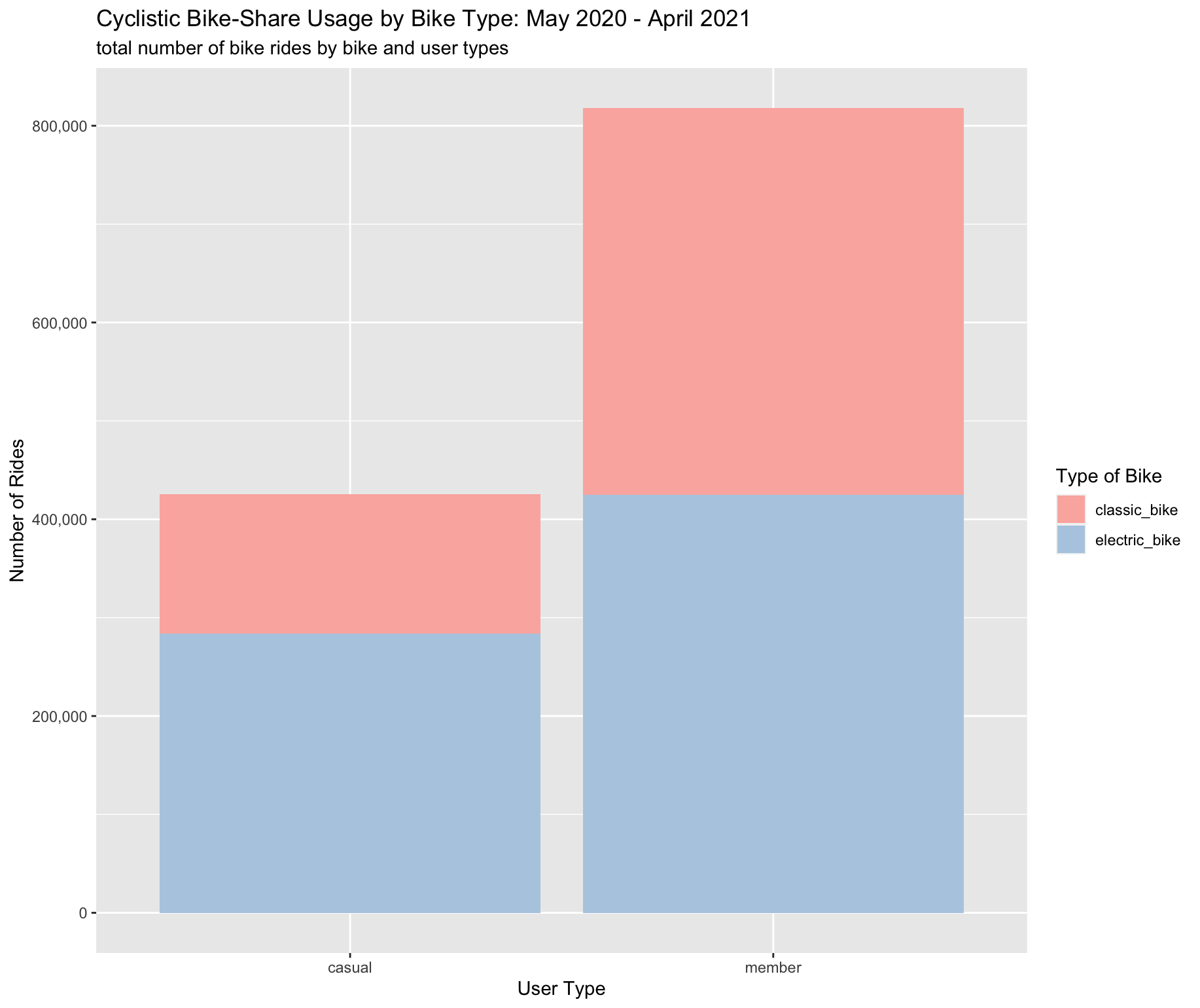
#`summarise()` has grouped output by 'member_casual'. You can override using the `.groups` argument.

## A tibble: 4 x 3
## Groups:   member_casual [2]
#  member_casual rideable_type number_of_rides
#  <chr>         <chr>                   <int>
#1 casual        classic_bike           141576
#2 casual        electric_bike          284024
#3 member        classic_bike           392911
#4 member        electric_bike          425068
Key Findings
Users with an annual membership complete more rides than casual riders
Among casual riders, Fridays, Saturdays, and Sundays are the most popular usage days
Casual riders, on average, spend about 76% more time on their rides than users with an annual membership
About 67% of total bike rides by casual riders were via electric bikes, compared to about 52% for total bike rides by users with an annual membership


Recommendations
Implement a new annual membership tier at a lower price point where a total number of rides are allotted for a given time period (e.g. week, month), versus current annual membership structure (unlimited number of rides, 45-min. limit per ride), and given that on average, casual riders spend more time on their rides than current members, but on average only 1480 sec.(24.67 min.)
Implement a limited time promotion for annual membership that loosens limits on Friday, Saturday, Sunday rides, given those are the most popular days casual riders use Cyclistic bikes
Add more electric bikes to inventory given casual riders prefer them over classic bikes
Other Considerations for Further Exploration
Collect data on available inventory at docking station user is at at point of rental to analyze impact on resulting bike type choice
Collect data on full route of a bike during rental, not just start and end locations, to analyze if certain areas/geospatial factors constitute certain bike types (e.g. terrain)
Include data on whether a casual rider uses a single-ride pass or full-day pass, to analyze how pricing may impact usage
View this case study on Kaggle